modelicares.linres¶

This submodule contains classes to help load, analyze, and plot results from Modelica linearizations:

• LinRes - Class to load, contain, and analyze results from a Modelica linearization
• LinResList - Specialized list of linearization results (LinRes instances)

class modelicares.linres.LinRes(fname='dslin.mat', tool=None)¶

Bases: modelicares._res.Res

Class for Modelica-based linearization results and methods to analyze those results

Initialization arguments:

• fname: Name of the file (including the directory if necessary)

  The file must contain four matrices: Aclass (specifies the class name, which must be “AlinearSystem”), nx, xuyName, and ABCD.

• tool: String indicating the linearization tool that created the file and thus the function to be used to load it

  By default, the available functions are tried in order until one works (or none do).

Methods:

• bode() - Create a Bode plot of the system’s response.
• nyquist() - Create a Nyquist plot of the system’s response.
• to_siso() - Return a SISO state-space system given input and output names.
• to_tf() - Return a transfer function given input and output names.

Properties:

• dirname - Directory from which the variables were loaded

• fbase - Base filename from which the variables were loaded, without the directory or extension

• fname - Filename from which the variables were loaded, with absolute path

• sys - State-space system as an instance of control.StateSpace

  It contains:

  • A, B, C, D: Matrices of the linear system

    der(x) = A*x + B*u;
         y = C*x + D*u;
    

  • state_names: List of names of the states (x)

  • input_names: List of names of the inputs (u)

  • output_names: List of names of the outputs (y)

• tool - String indicating the function used to load the results (named after the corresponding Modelica tool)

Example:

>>> lin = LinRes('examples/PID.mat')
>>> print(lin) 
Modelica linearization results from .../examples/PID.mat

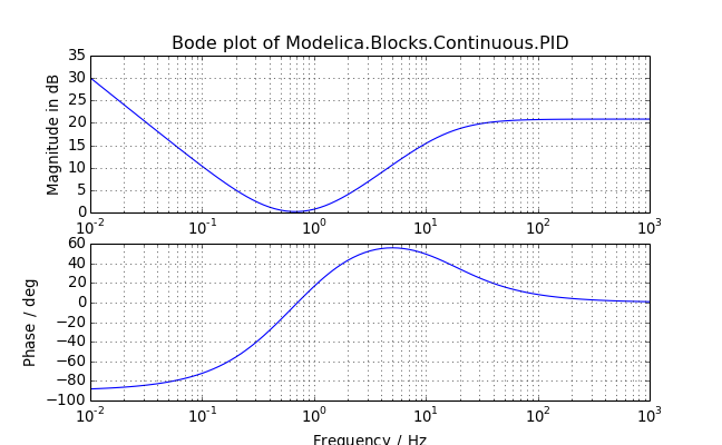
bode(axes=None, pairs=None, label='bode', title=None, colors=['b', 'g', 'r', 'c', 'm', 'y', 'k'], styles=[(None, None), (3, 3), (1, 1), (3, 2, 1, 2)], **kwargs)¶

Create a Bode plot of the system’s response.

The Bode plots of a MIMO system are overlayed. This is different than MATLAB^®, which creates an array of subplots.

Arguments:

• axes: Tuple (pair) of axes for the magnitude and phase plots

  If axes is not provided, then axes will be created in a new figure.

• pairs: List of (input name or index, output name or index) tuples of each transfer function to be evaluated

  By default, all of the transfer functions will be plotted.

• label: Label for the figure (ignored if axes is provided)

  This is used as the base filename if the figure is saved using save() or saveall().

• title: Title for the figure

  If title is None (default), then the title will be “Bode plot of fbase”, where fbase is the base filename of the data. Use ‘’ for no title.

• colors: Color or list of colors that will be used sequentially

  Each may be a character, grayscale, or rgb value.

  See also

  http://matplotlib.sourceforge.net/api/colors_api.html

• styles: Line/dash style or list of line/dash styles that will be used sequentially

  Each style is a string representing a linestyle (e.g., ‘–’) or a tuple of on/off lengths representing dashes. Use ‘’ for no line or ‘-‘ for a solid line.

  See also

  http://matplotlib.sourceforge.net/api/collections_api.html

• **kwargs: Additional plotting arguments:

  • freqs: List or frequencies or tuple of (min, max) frequencies over which to plot the system response.

    If freqs is None, then an appropriate range will be determined automatically.

  • in_Hz: If True (default), the frequencies (freqs) are in Hz and should be plotted in Hz (otherwise, rad/s)

  • in_dB: If True (default), plot the magnitude in dB

  • in_deg: If True (default), plot the phase in degrees (otherwise, radians)

  Other keyword arguments are passed to matplotlib.pyplot.plot().

Returns:

1. axes: Tuple (pair) of axes for the magnitude and phase plots

Example:

(Source code, png, hires.png, pdf)

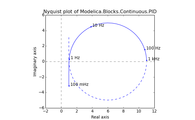
nyquist(ax=None, pairs=None, label='nyquist', title=None, xlabel='Real axis', ylabel='Imaginary axis', colors=['b', 'g', 'r', 'c', 'm', 'y', 'k'], **kwargs)¶

Create a Nyquist plot of the system’s response.

The Nyquist plots of a MIMO system are overlayed. This is different than MATLAB^®, which creates an array of subplots.

Arguments:

• ax: Axes onto which the Nyquist diagram should be plotted

  If ax is not provided, then axes will be created in a new figure.

• pairs: List of (input name or index, output name or index) tuples of each transfer function to be evaluated

  By default, all of the transfer functions will be plotted.

• label: Label for the figure (ignored if ax is provided)

  This is used as the base filename if the figure is saved using save() or saveall().

• title: Title for the figure

  If title is None (default), then the title will be “Nyquist plot of fbase”, where fbase is the base filename of the data. Use ‘’ for no title.

• xlabel: x-axis label

• ylabel: y-axis label

• colors: Color or list of colors that will be used sequentially

  Each may be a character, grayscale, or rgb value.

  See also

  http://matplotlib.sourceforge.net/api/colors_api.html

• **kwargs: Additional plotting arguments:

  • freqs: List or frequencies or tuple of (min, max) frequencies over which to plot the system response.

    If freqs is None, then an appropriate range will be determined automatically.

  • in_Hz: If True (default), the frequencies (freqs) are in Hz and should be plotted in Hz (otherwise, rad/s)

  • mark: True, if the -1 point should be marked on the plot

  • show_axes: True, if the axes should be shown

  • skip: Mark every nth frequency on the plot with a dot

    If skip is 0 or None, then the frequencies are not marked.

  • label_freq: If True, if the marked frequencies should be labeled

  Other keyword arguments are passed to matplotlib.pyplot.plot().

Returns:

1. ax: Axes of the Nyquist plot

Example:

(Source code, png, hires.png, pdf)

to_siso(iu=None, iy=None)¶

Return a SISO system given input and output indices.

Arguments:

• iu: Index or name of the input

  This must be specified unless the system has only one input.

• iy: Index or name of the output

  This must be specified unless the system has only one output.

Example:

>>> lin = LinRes('examples/PID.mat')
>>> lin.to_siso()
A = [[   0.    0.]
 [   0. -100.]]

B = [[   2.]
 [ 100.]]

C = [[  1. -10.]]

D = [[ 11.]]

to_tf(iu=None, iy=None)¶

Return a transfer function given input and output names.

Arguments:

• iu: Index or name of the input

  This must be specified unless the system has only one input.

• iy: Index or name of the output

  This must be specified unless the system has only one output.

Example:

>>> lin = LinRes('examples/PID.mat')
>>> lin.to_tf()
(array([[  11.,  102.,  200.]]), array([   1.,  100.,    0.]))

class modelicares.linres.LinResList(*args)¶

Bases: modelicares._res.ResList

Specialized list of linearization results

Initialization signatures:

• LinResList(): Returns an empty linearization list

• LinResList(lins), where lins is a list of LinRes instances: Casts the list into a LinResList

• LinResList(filespec), where filespec is a filename or directory, possibly with wildcards a la glob: Returns a LinResList of LinRes instances loaded from the matching or contained files

  The filename or directory must include the absolute path or be resolved to the current directory.

  An error is only raised if no files can be loaded.

• LinResList(filespec1, filespec2, ...): Loads all files matching or contained by filespec1, filespec2, etc. as above.

  Each file will be opened once at most; duplicate filename matches are ignored.

Built-in methods:

The entries are LinRes instances, but linearizations can be specified via filename when initializing or appending the list. The list has all of the methods of a standard Python list (e.g., + or __add__/__radd__, clear(), in or __contains__, del or __delitem__, __getitem__, += or __iadd__, *= or __imul__, iter() or __iter__, copy(), extend(), index(), insert(), len() or __len__, * or __mul__/__rmul__, pop(), remove(), reverse(), reversed() or __reversed__, = or __setitem__, __sizeof__(), and sort()). By default, the sort() method orders the list of linearizations by the full path of the result files.

Overloaded methods:

• append() - Add linearization(s) to the end of the list of linearizations (accepts a LinRes instance, directory, or filename).

Additional methods:

• bode() - Plot the linearizations onto a single Bode diagram.
• nyquist() - Plot the linearizations onto a single Bode diagram.

Properties:

• basedir - Highest common directory that the result files share
• Also, the properties of LinRes (basename, dirname, fname, sys, and tool) can be retrieved as a list across all of the linearizations; see the example below.

Example:

>>> lins = LinResList('examples/PID/*/')
>>> lins.dirname 
['.../examples/PID/1', '.../examples/PID/2']

append(item)¶

Add linearization(s) to the end of the list of linearizations.

Arguments:

• item: LinRes instance or a file specification

  The file specification may be a filename or directory, possibly with wildcards a la glob, where linearization results can be loaded by LinRes. The filename or directory must include the absolute path or be resolved to the current directory. An error is only raised if no files can be loaded.

Unlike the append method of a standard Python list, this method may add more than one item. If item is a directory or a wildcarded filename, it may match multiple valid files.

Linearization results will be appended to the list even if they are already included.

Example:

>>> lins = LinResList('examples/PID/*/')
>>> lins.append('examples/PID.mat')
>>> print(lins) 
List of linearization results (LinRes instances) from the following files
in the .../examples directory:
   PID/1/dslin.mat
   PID/2/dslin.mat
   PID.mat

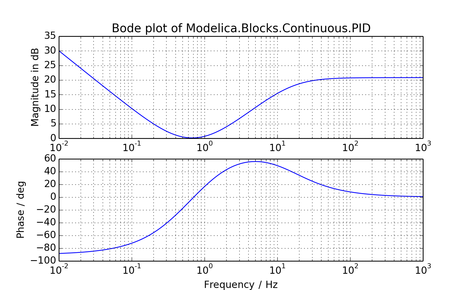
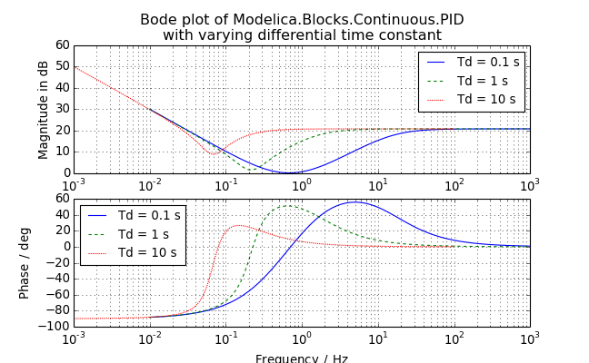
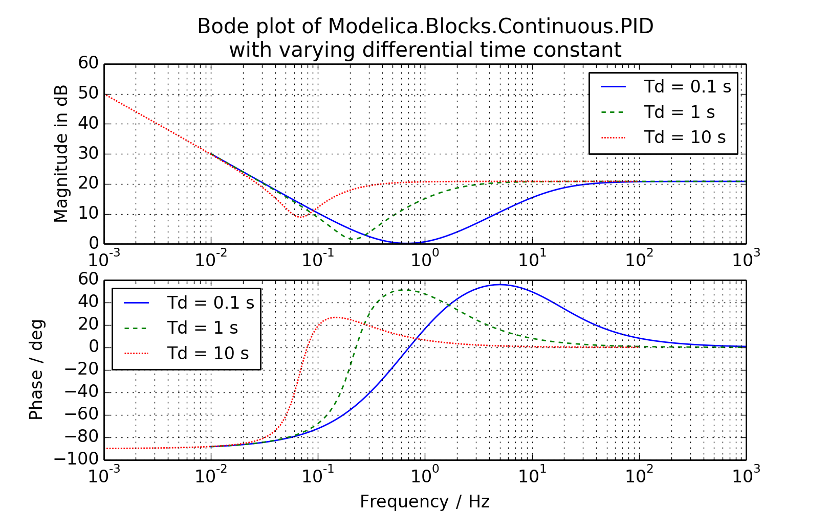
bode(axes=None, pair=(0, 0), label='bode', title='Bode plot', labels=None, colors=['b', 'g', 'r', 'c', 'm', 'y', 'k'], styles=[(None, None), (3, 3), (1, 1), (3, 2, 1, 2)], leg_kwargs={}, **kwargs)¶

Plot the linearizations onto a single Bode diagram.

This method calls LinRes.bode() from the included instances of LinRes.

Arguments:

• axes: Tuple (pair) of axes for the magnitude and phase plots

  If axes is not provided, then axes will be created in a new figure.

• pair: Tuple of (input name or index, output name or index) for the transfer function to be chosen from each system (applied to all)

  This is ignored if the system is SISO.

• label: Label for the figure (ignored if axes is provided)

  This is used as the base filename if the figure is saved using save() or saveall().

• title: Title for the figure

• labels: Label or list of labels for the legends

  If labels is None, then no label will be used. If it is an empty string (‘’), then the base filenames will be used.

• colors: Color or list of colors that will be used sequentially

  Each may be a character, grayscale, or rgb value.

  See also

  http://matplotlib.sourceforge.net/api/colors_api.html

• styles: Line/dash style or list of line/dash styles that will be used sequentially

  Each style is a string representing a linestyle (e.g., ‘–’) or a tuple of on/off lengths representing dashes. Use ‘’ for no line and ‘-‘ for a solid line.

  See also

  http://matplotlib.sourceforge.net/api/collections_api.html

• leg_kwargs: Dictionary of keyword arguments for matplotlib.pyplot.legend()

  If leg_kwargs is None, then no legend will be shown.

• **kwargs: Additional plotting arguments:

  • freqs: List or frequencies or tuple of (min, max) frequencies over which to plot the system response.

    If freqs is None, then an appropriate range will be determined automatically.

  • in_Hz: If True (default), the frequencies (freqs) are in Hz and should be plotted in Hz (otherwise, rad/s)

  • in_dB: If True (default), plot the magnitude in dB

  • in_deg: If True (default), plot the phase in degrees (otherwise, radians)

  Other keyword arguments are passed to matplotlib.pyplot.plot().

Returns:

1. axes: Tuple (pair) of axes for the magnitude and phase plots

Example:

(Source code, png, hires.png, pdf)

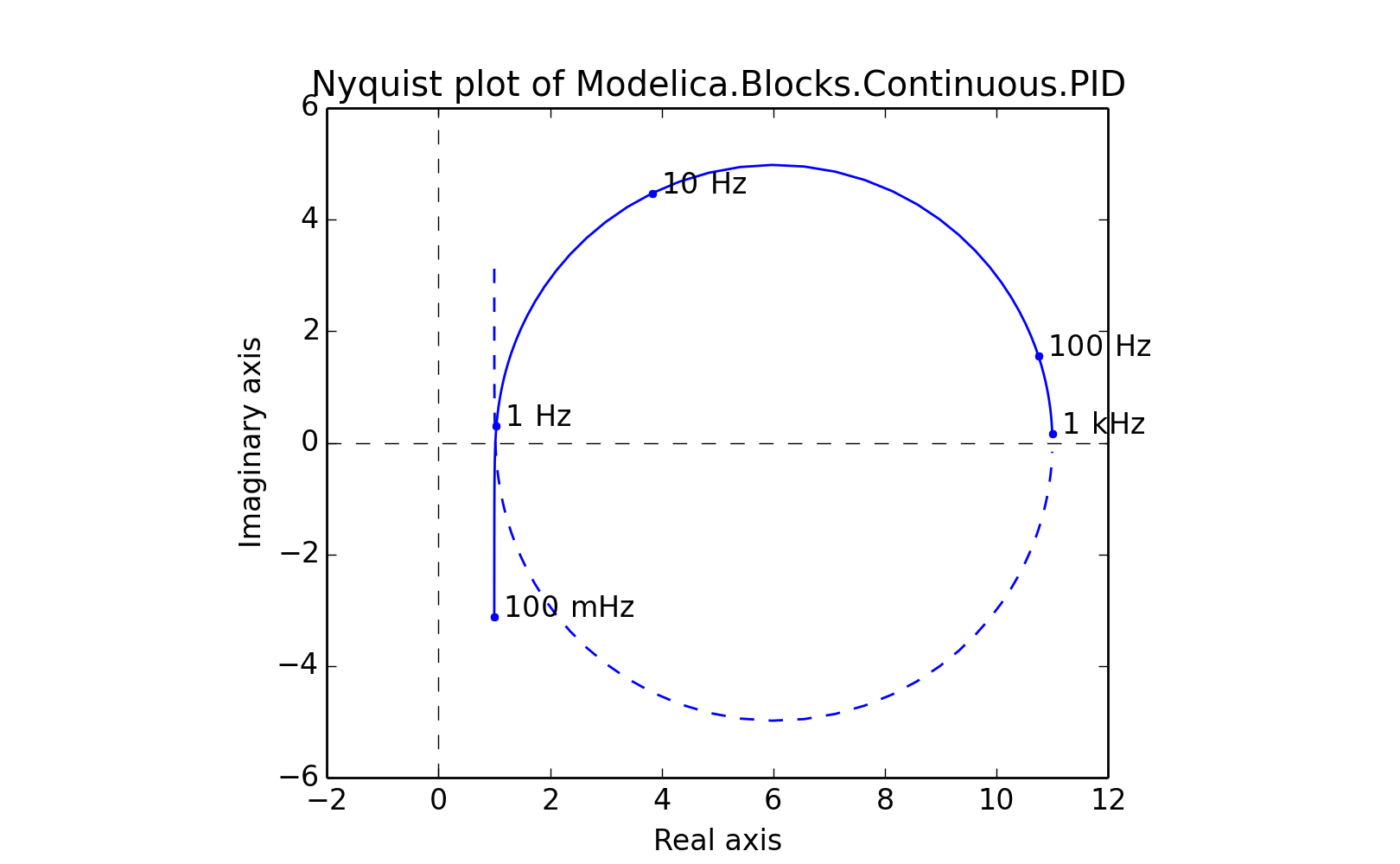
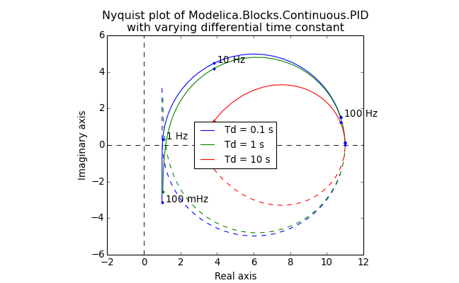
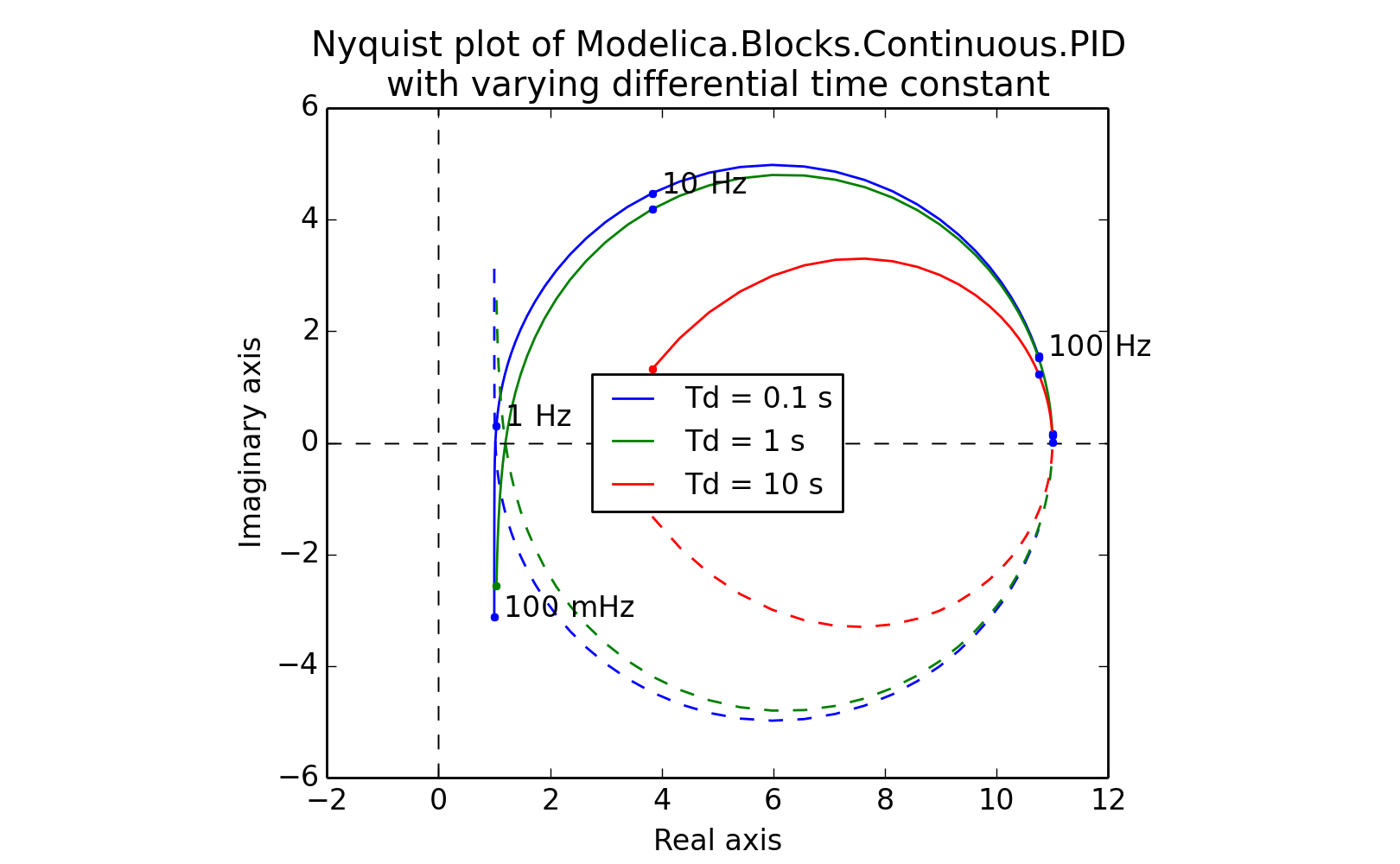
nyquist(ax=None, pair=(0, 0), label='nyquist', title='Nyquist plot', xlabel='Real axis', ylabel='Imaginary axis', labels=None, colors=['b', 'g', 'r', 'c', 'm', 'y', 'k'], leg_kwargs={}, **kwargs)¶

Plot the linearizations onto a single Nyquist diagram.

This method calls nyquist() from the included instances of LinRes.

Arguments:

• ax: Axes onto which the Nyquist diagrams should be plotted

  If ax is not provided, then axes will be created in a new figure.

• pair: Tuple of (input name or index, output name or index) for the transfer function to be chosen from each system (applied to all)

  This is ignored if the system is SISO.

• label: Label for the figure (ignored if axes is provided)

  This is used as the base filename if the figure is saved using save() or saveall().

• title: Title for the figure

  • xlabel: x-axis label
  • ylabel: y-axis label

• labels: Label or list of labels for the legends

  If labels is None, then no label will be used. If it is an empty string (‘’), then the base filenames will be used.

• colors: Color or list of colors that will be used sequentially

  Each may be a character, grayscale, or rgb value.

  See also

  http://matplotlib.sourceforge.net/api/colors_api.html

• leg_kwargs: Dictionary of keyword arguments for matplotlib.pyplot.legend()

  If leg_kwargs is None, then no legend will be shown.

• **kwargs: Additional plotting arguments:

  • freqs: List or frequencies or tuple of (min, max) frequencies over which to plot the system response.

    If freqs is None, then an appropriate range will be determined automatically.

  • in_Hz: If True (default), the frequencies (freqs) are in Hz and should be plotted in Hz (otherwise, rad/s)

  • mark: True, if the -1 point should be marked on the plot

  • show_axes: True, if the axes should be shown

  • skip: Mark every nth frequency on the plot with a dot

    If skip is 0 or None, then the frequencies are not marked.

  • label_freq: If True, if the marked frequencies should be labeled

  Other keyword arguments are passed to matplotlib.pyplot.plot().

Returns:

1. ax: Axes of the Nyquist plot

Example:

(Source code, png, hires.png, pdf)